Why so much hate against propensity score matching?

I’ve seen several variants of this meme on Twitter recently.

https://twitter.com/HallaMartin/status/1090025805764276225

This is just one example, so nothing against @HallaMartin. But his tweet got me thinking. Apparently, in the year 2019 it’s not possible anymore to convince people in an econ seminar with a propensity score matching (or any other matching on observables, for that matter). But why is that?

Here’s what I think. The typical matching setup looks somewhat like this:

You’re interested in estimating the causal effect of X on Y. But in order to do so, you will need to adjust for the confounders W, otherwise you’ll end up with biased results. If you’re able to measure W, this adjustment can be done in a propensity score matching, which is actually an efficient way of dealing with a large set of covariates.

The problem though is to be sure that you’ve adjusted for all possible confounding factors. How can you be certain that there are no unobserved variables left that affect both X and Y? Because if the picture looks like the one below (where the unobserved confounders are depicted by the dashed bidirected arc), matching will only give you biased estimates of the causal effect you’re after.

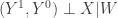
Presumably, the Twitter meme is alluding to exactly this problem. And I agree that it’s hard to make the claim that you’ve accounted for all confounding influence factors in a matching. But how’s that with economists’ most preferred alternative—the instrumental variable (IV) estimator? Here the setup looks like this:

Now, unobserved confounders between X and Y are allowed, as long as you’re able to find an instruments Z that affects X, but which doesn’t affect Y directly (other than through X). In that case, Z creates exogenous variation in X that can be leveraged to estimate X‘s causal effect. (Because of the exogonous variation in X induced by Z, we also call this IV setup a surrogate experiment, by the way.)

Great, so we have found a way forward if we’re not 100% sure that we’ve accounted for all unobserved confounders. Instead of a propensity score matching, we can simply resort to an IV estimator.

But if you think about this a bit more, you’ll realize that we face a very similar situation here. The whole IV strategy breaks down if there are unobserved confounders between Z and Y (see again the dashed arc below). How can we be sure to rule out all influence factors that jointly affect the instrument and the outcome? It’s the same problem all over again.

So in that sense, matching and IV are not very different. In both cases we need to carefully justify our identifying assumptions based on the domain knowledge we have. Whether ruling out is more plausible than depends on the specific context under study. But on theoretical grounds, there’s no difference in strength or quality between the two assumptions. So I don’t really get why—as a rule—economists shouldn’t trust a propensity score matching, but an IV approach is fine.

Now you might say that this is just Twitter babble. But my impression is that most economists nowadays would be indeed very suspicious towards “selection on observables”-types of identification strategies.* Even though there’s nothing inherently implausible about them.

In my view, the opaqueness of the potential outcome (PO) framework is partly to blame for this. Let me explain. In PO you’re starting point is to assume uncofoundedness of the treatment variable

.

This assumption requires that the treatment X needs to be independent of the potential outcomes of Y, when controlling for a vector of covariates W (as in the first picture above). But what is this magic vector W that can make all your causal effect estimation dreams come true? Nobody will tell you.

And if the context you’re studying is a bit more complicated than in the graphs I’ve showed you—with several causally conected variables in a model—it’ becomes very complex to even properly think this through. So in the end, deciding whether unconfoundedness holds becomes more of guessing game.

My hunch is that after having seen too many failed attempts of dealing with this sort of complexity, people have developed a general mistrust against unconfoundedness and strong exogeneity type assumptions. But we still don’t want to give up on causal inference altogether. So we move over to the next best thing: IV, RDD, Diff-in-Diff, you name it.

It’s not that these methods have weaker requirements. They all rely on untestable assumptions about unobservables. But maybe they seem more credible because you’ve jumped through more hoops with them?

I don’t know. And I don’t want to get too much into kitchen sink psychology here. I just know that the PO framework makes it incredibly hard to justify crucial identification assumptions, because it’s so much of a black box. And I think there are better alternatives out there, based on the causal graphs I used in this post (see also here). Who knows, maybe by adopting them we might one day be able to appreciate a well carried out propensity score matching again.

---

* Interestingly though, this only seems to be the case for reduced-form analyses. Structural folks mostly get away with controlling for observables; presumably because structural models make causal assumptions much more explicit than the potential outcome framework.