Last week I was teaching about graphical models of causation at a summer school in Montenegro. You can find my slides and accompanying R code in the teaching section of this page. It was lots of fun and I got great feedback from students. After the workshop we had stimulating discussions about the usefulness of this new approach to causal inference in economics and business. I’d like to pick up one of those points here, as this is an argument I frequently hear when talking to people with a classical econometrics training.
PhD students in economics are usually well-trained in the potential outcome framework. Therefore, I mostly frame directed acyclic graphs (DAG) as a useful complement to the standard treatment effects estimators, in order to conceal my true revolutionary motives. ;) One concern with DAGs I sometimes encounter though is that they require so many strong assumptions about the presence (and absence) of causal relationships between variables in your model. By contrast, so the argument goes, for treatment effect estimators, such as nearest-neighbor matching, you only have to justify the exogeneity of your treatment and that’s it. No need to specify a full causal model.
This argument is misguided. You always need a “full” causal model in order to do proper causal inference. But let me specify in more detail what I mean by this. In matching (or inverse probability weighting, or regression, or any other method that relies on unconfoundedness) you encounter a situation like the following. 
You would like to estimate the effect of a treatment T (e.g., an R&D subsidy) on an outcome variable Y (e.g., firm growth). The problem is that there are other variables, X, out there that create a correlation between the treatment and outcome. You first need to control for these confounding factors in order to get at the true causal effect of T on Y.
In the potential outcome framework this means that you need to justify the unconfoundedness assumption.
If the treatment is independent of potential outcomes conditional on X—and you’re able to measure all these influence factors X—then you’re fine. The crux though is, what is X? Which variables do you need to control for? And what other influence factors can you safely keep uncontrolled for? To make these claims you need to have a causal model—at least in your mind. And here the circle closes.
Every time you estimate something that entails the unconfoundedness assumption, you imply that your data is generated by a causal process such as the one depicted above. So treatment effects estimators don’t require fewer assumptions than graphical approaches, they just apply for one very specific causal model. If that model fits reality, great! Then you can go out and apply treatment effects methods “off the shelf”. But if it doesn’t you need to think harder about an appropriate model. And DAGs offer you a tremendously useful tool set to handle these types of situations.
Here’s the causal model that applies for the second most prominent estimator from the treatment effects literature—the non-parametric IV estimator.

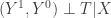
In this situation there is no possibility of ever controlling for all confounding influences, because some of them remain unobserved (denoted by the dashed bidirected arc between T and Y). As a result, unconfoundedness will be violated. But instead you can do something else. You can use variation in a third variable Z to get at the causal effect of T on Y.¹ In order for that to work, you have to satisfy a very similar condition to unconfoundedness for the instrument though.
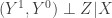
Your instrument has to be excludable, or independent of potential outcomes given a vector of control variables X. You see that you’re basically left with the same problem. How do you decide what is in X, and what isn’t?
In sum, treatment effects estimators such as matching and IV simply give you a template of a causal model at hand. If this template describes reality accurately you can easily find causal effect estimates with the help of standard techniques. Graphical models capture the same standard cases, but on top of that provide you with a much more versatile toolbox for causal inference. The impression that matching and IV require fewer assumptions is a misconception. I admit it’s probably still easier to convince reviewers with the standard methods, simply because we’re so used to them. But that’s just a sign for an imperfection of the scientific process and says nothing about any substantive differences between both approaches. Causal inference requires strong assumptions, one way or the other. There is no such thing as a free lunch in econometrics either.
¹ In addition, you will need to assume monotonicity, i.e., a monotone influence of Z on T for all members in the population. And even then, you can only identify an effect for a subgroup of compliers, that changes their treatment status due to the instrument (for binary Z). These details are of secondary importance for the argument here. If you’re interested you can check the seminal paper by Imbens and Angrist (1994) on nonparaemtric IV.

Interesting topic, Paul, and indeed a very nice discussion that we started there in Montenegro.
However, while generally most any econometric technique of causal inference relies on assumptions for identification (e.g. the one of steady-state systems or that our causal models do not entail out of equilibrium predictions), I disagree with you to the extent that I think that the kind of assumptions you find behind DAGs are stronger compared to those that (most) treatment effect estimation techniques build on.
To make this clearer, let’s start from the benchmark case for any study making a causal inference claim. Consider, for instance, that I would want to assess the effect of a certain “pill” on a candidate. Ideally, one would randomly select candidates into treated and control (+ maybe placebo) groups. The true beauty of randomization is that (for sufficiently large groups), all unobservable (and observable) confounders will be equally distributed among groups, so that we are able to control for the observables directly and for all unobservables at the mean of the sampled population. Hence, we are able to estimate an (isolated) true causal effect at the average of the treated, without having to be aware of the underlying full causal model in place.
A well-known and well-experienced problem, however, is that usually as econometricians we are not able to manipulate the system of agents we are studying (there are some exceptions, but this is not the norm) and assign treatments at random. Therefore, we have to approximate such ideal experimental conditions by identifying and exploiting natural, i.e. given, sources of de facto randomization. The admittedly least creative way of doing this is to use matching; Here the idea is to group pairs of treated and non-treated candidates which are so highly comparable in a way that the occurrence of the treatment can be considered as being quasi random. To me this works a bit like reverse engineering of the ideal experimental approach. However, matching is problematic with regards to identification of causal effects and often misleading. This because for a true causal effect estimation it would require the researcher to be, first of all, aware of and, second, able to match on all confounders in the relationship of interest – which, at least in my view, seems quite unrealistic. As such, matching techniques rely on the same (or at least similarly) strong assumptions as DAGs. Frequently we see matching used in combination with a conditional or fully blocked natural experiment within a differences-in-differences setting. This appears reasonable in the presence of any time varying confounders. Very often, however, people “abuse” matching in such settings where the treatment occurrence is de facto not random, in the attempt to calibrate the trial. At the bottom line, this will result in making the same strong assumption as in the previous cases, as matching is in the end nothing more than a non-parametric control approach, for only observables available.
But how about the more “premium” treatment effect estimation techniques, namely IV or differences-in-differences with a natural experiment? These techniques exploit sources of actual exogenous variation, i.e. random shocks, in the causal system in order to approximate a randomized trial. Good examples of such exogenous shifters include the aforementioned Vietnam lottery or, unexpected, premature deaths or rainfall.
Do these techniques rely on less strong assumptions than DAGs or matching? The answer is: yes! And here is why: As mentioned above, under random assignment, the researcher does not have to be entirely aware of the full causal model, as the mass of unobserved confounding X’s will be controlled for at the mean of the sampled groups (which is limiting but still a good deal considering that we are able to estimate a true causal effect). With this in mind, it becomes clear that in the case of IV/ natural experiments the mere assumption that researcher has to credibly defend for causal identification is the one of pure exogeneity of the instrument (* again monotonicity aside, which might be indeed an issue in some of the cases). But most importantly, – unlike in DAGs and matching – here we are able to falsify our assumptions, as we actually dispose of a candidate random shifter. In other words, it is much less far-fetched to assume that I can find any (at least one) X that might confute the randomness of my treatment compared to assuming that I can find all X’s that impact the causal relationship between T and Y.
Given the significant potential for philosophical escalation there is to this discussion, this appears as a fundamental difference when it comes to weighting the strength of assumptions to be made in these techniques vis-à-vis. However, by no means does this imply that treatment effect estimation is an ‘easy way out’ – quite the opposite; Justifying the randomness of a shock and validating an instrument requires an extreme amount of rigor and does not allow to take shortcuts. E.g., real world lotteries will have defiers, rainfall will be seasonal, and more prolific or extrovert people might be more likely to die unexpectedly – there goes our validity. For some of these concerns we can test, others are so severe that we need to find other instruments or define them differently. And this is tedious. Because, yes, there is indeed no such thing as a free lunch in causal inference.
LikeLike
Hi Thomas! I really like this discussion and appreciate that you took the time to write down your thoughts. :)
The Vietnam lottery paper is indeed a great example. Although the draft appears to be plausibly exogenous (the word ‘lottery’ already implies it), the instrument got later criticized by (if I remember correctly) Heckman who argued that employers who observe draft outcomes might invest less in the human capital of their drafted employees. Such a mechanism would undermine identification because “training employees” acts as a post-treatment confounder and opens up the path Z -> X -> Y (Z: draft lottery, X: training, Y: wage). My point is, how do you settle this debate? Angrist will argue that the path Z -> X -> Y is absent, whereas Heckman will doubt that claim. But while bringing forward these arguments both have essentially just drawn a DAG in their head (or formulated a model about the DGP, to express it in terms more familiar to economists). I mean it in that sense when I say that DAGs, as a method, do not require stronger assumptions for causal inference than treatment effect estimators based on the potential outcome framework (both frameworks are equivalent anyways).
DAGs are just a language to make the assumptions that are necessary for causal inference explicit; their strength will be the same in the end however. But of course there are certain settings where you have so much control over or knowledge about the DGP (e.g., in an RCT or RDD) that these assumptions are very credible, and others where they aren’t (e.g., simple covariate adjustment for a highly endogenous treatment). The point is that DAGs can capture all these cases too. That’s what makes them so flexible.
The treatment effect literature essentialy gives you three standard templates at hand (RCT, matching based on simple confounding, IV; RDD is a special case of the latter) and researchers need to (often artificially) make their setting fit to them. DAGs, by contrast, provide you with the full range of settings in which causal effects are identifiable in non-parametric, recursive models. Thus, if you can justify causal inference with treatment effects estimators, you can justify them in DAGs too (with the addition of monotonicty for IV). At the same time, however, there are many more situations that don’t fit the standard treatment effects templates, but where causal effects can be identified based on DAGs.
LikeLike
Hi Thomas,
Do you recommend any textbook(s) to get more familiar with the topics you discussed in your reply? I read Judea Pearls Causality Textbook but I am not sure where to start with the economists perspective.
Thank you
LikeLike
Scott Cunningham has a nice section in his Econometrics Mixtape on DAG’s where he shows how graphical representations of causal effects can be very helpful to teach research designs and estimators. For example, IV’s have a very intuitive DAG representation. So, definitely DAG’s cannot replace IV’s or natural experiments (similar to matching; today, no one with some experience with matching methods will claim causality based on matching alone due to the reasons Thomas mentioned already), but they can be very nice complements.
LikeLike
Hi Jeroen! I know Scott’s Mixtape and agree that it’s a great resource to teach econometrics in a modern, more conceptual and less statistics-focussed way. I’m not completely sure though what you mean by “DAGs replacing IV”. My point was that the IV setting (as well as matching) is just a special case of what graphical models can capture. If your model of the data generating process fits the “IV template” then you can go ahead and apply standard techniques (if you’re willing to assume linearity or monotonicity on top). But what I see in practice is unfortunately the opposite. People have a template (IV or matching) and try to make their data generating process fit to it (essentially by hand-waving). Here DAGs offer much more flexibility. The strength of the assumptions you need to impose is exactly the same, DAGs just make them more explicit than if you use off-the-shelf methods.
LikeLike
Thanks for great explanation! May I ask you a question? Let us assume that after conditioning on family SES, a researcher did not find any significant net effects of private school on student academic achievement. He thus strongly concluded that with respect to student academic achievement, private school effects are primarily function of family SES. Are there any reasons to suspect his claim? It seems clear that family SES is an important confounder between school types and academic achievement.
LikeLike
Hi Paul, thanks for your feedback! I’m not an expert in education/labor but it sounds plausible to me. Let’s assume we have a simple graph with two paths. The first is: private school -> academic achievement. And a second confounding path is: private school academic achievement. After conditioning on family SES, no effect on the main causal path is detectable, while there was a positive correlation before. This corrletaion could have been due to a positive causal effect of family SES on private school attendance, coupled with a positive effect of family SES on academic achievement. To me, this is the most plausible explanation. Technically it could be the other way round too though. If family SES exerts a negative effect on both private school attendance and academic achievement, this could also produce a positive correlation on the confounding path. And if your graph is more complicated than the simple one I layed out here, many more things can happen of course. So this is another great example for how the interpretation of empirical results crucially depends on the model (i.e., graph) you impose on the data.
LikeLike