Econometrics and the “not invented here” syndrome: suggestive evidence from the causal graph literature

[This post requires some knowledge of directed acyclic graphs (DAG) and causal inference. Providing an introduction to the topic goes beyond the scope of this blog though. But you can have a look at a recent paper of mine in which I describe this method in more detail.]

Graphical models of causation, most notably associated with the name of computer scientist Judea Pearl, received a lot of pushback from the grandees of econometrics. Heckman had his famous debate with Pearl, arguing that economics looks back on its own tradition of causal inference, going back to Haavelmo, and that we don’t need DAGs. Here’s a quote from a paper by Guido Imbens in Statistical Science making a similar point:

“In contrast, the causal graphs have not caught on in economics. In my view a major reason is that there have been few compelling applications of causal graphs to social science questions where the causal-graph approach has generated novel analyses or prevented researchers from making mistakes that other frameworks might have encouraged them to make.”

Pearl largely attributes this attitude to a form of “not invented here” syndrome. At least you get this impression while reading this funny exchange between him and Imbens on Pearl’s “causality blog”.

To flesh out one of Imbens’ points in more detail, think about the assumption of unconfoundedness in the treatment effect literature,

which states that a treatment variable T is independent of potential outcomes given a set of controls X. Related to the quote I gave, Imbens questions whether DAGs can help economists to decide about which variables to include in X, and which to leave out. He believes they don’t.

Well, I firmly stand on Pearl’s side in this debate and think that DAGs can actually help a great deal here. I’ll try to give you a concrete example from economics. Here’s a passage from Angrist and Pischke’s “bad control” chapter in Mostly Harmless Econometrics:

“Suppose we are interested in the effects of a college degree on earnings and that people can work in one of two occupations, white collar and blue collar. A college degree clearly opens the door to higher-paying white collar jobs. Should occupation therefore be seen as an omitted variable in a regression of wages on schooling? After all, occupation is highly correlated with both education and pay. Perhaps it’s best to look at the effect of college on wages for those within an occupation, say white collar only. The problem with this argument is that once we acknowledge the fact that college affects occupation, comparisons of wages by college degree status within an occupation are no longer apples-to-apples, even if college degree completion is randomly assigned.”

So you should not control for occupation in this example. But why? Angrist and Pischke provide a—somewhat convoluted—argument based on the potential outcome framework.¹ But to be honest, I always had a hard time to follow their chapter here.² By contrast, DAGs make things a lot easier. Under unconfoundedness we have a situation like this (pictures produced by DAGitty):

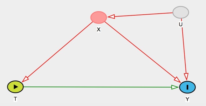
X affects both the treatment and outcome variable, but once we control for it (given that we can measure it) we’re fine—unconfoundedness holds. The presence of an unobserved confounder U doesn’t matter in this case. By contrast, Angrist and Pischke have a situation like this in mind:

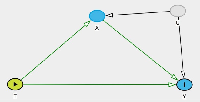
Only a tiny detail has changed, namely that the causal link between T and X now goes in the other direction. College education (T) affects your future occupation (X), which in turn affects your future income (Y). Suddenly, controlling for X causes problems. It opens up the causal path going through U (, because X is a collider on that path) and produces bias. The unobsorved confounder U in Angrist and Pischke’s example, by the way, is the infamous ability³ variable, which becomes clear if you read their footnote:

“In this example, selection bias is probably negative […]. It seems reasonable to think that any college graduate can get a white collar job […]. But someone who gets a white collar without benefit of a college degree […] is probably special, i.e., has a better than average .”

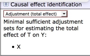
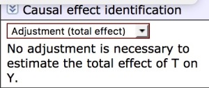
The point is, DAGs help a lot in this example to understand where the problem exactly comes from. Pearl’s do-calculus immediately tells you, based on the graph, whether you should control for X or not. DAGitty does so too (not surprising, as it’s based on do-calculus). In situation 1:

And in situation 2:

Afterwards, DAGs also make it easy to share this knowledge with your audience. In the potential outcome framework, on the other hand, things are much more opaque.

Ironically, in economics, reduced-form people like Imbens get a lot of criticism from structural folks. Structuralists would argue that starting from an assumption like unconfoundedness is really a black-box, and that we need to make explicit the underlying model on which we base our judgement (I’d say Heckman is in this camp too, for example). DAGs are a convenient tool to achieve exactly that. Suddenly, unconfoundedness becomes a corollary, deduced from substantive knowledge encoded in the graph, rather than a mere assumption. At the same time, graphs are more easily communicated—and frankly intuitive—than algebraic propositions. Another reasons why I strongly believe we should include them in our econometric toolbox.

To quote Imbens once more:

“I see substantial evidence that as a group economists are willing to adopt new methods from other disciplines that are viewed as useful in practice.”

If that’s true (and I sincerely hope so), let’s maybe stop pushing back so hard against graphical models of causation and give the method a real chance.

By the way: the title of this post is a joke, of course. :)

---

¹ Yes, it’s possible to make this argument in the potential outcome framework. This is one point Imbens stresses in his debate with Pearl on the causality blog. It’s just neither very convenient nor instructive, I think.

² Following is probably not so much the problem, but to get an intuitive understanding of the argument such that I can apply it in different contexts in my own research.

³ Infamous, because “ability” seems to be the knee-jerk source of endogeneity in many economic settings.